Quickstart

mwave is a python library designed to help explore new matterwave interferometer geometries. mwave also provides functions to numerically solve the Hamiltonian that describes Bragg diffraction and Bloch oscillations.

Installation

Stable releases of mwave can be downloaded from Github or via:

pip install git+https://github.com/jc-roth/mwave@v3.0.0

A first example

Defining an interferometer geometry

mwave is losely broken up into three parts: a module for symbolically defining arbitrary interferometer geometries, a module for numerically defining arbitrary interferometer geometries, and a module for numerically integrating Bragg and Bloch processes. As an example we will use the library to explore a Mach-Zender interferometer geometry.

First we will import the required libraries

from mwave import symbolic as msym
from mwave import integrate as mint
import numpy as np
import sympy as sp
from matplotlib import pyplot as plt

mwave internally uses the sympy library to build symbolic expressions of the interferometer phase. Therefore we must define the symbols we want to use symbolically

m, c, hbar, k, g, delta, n, T, t_traj = sp.symbols('m c hbar k g delta n T t_traj', real=True)
k_eff = 2*k

Performing certain operations in mwave requires the user to set certain constants. In this example we will need to set the mass, speed of light, the Planck constant, and another variable called t_traj.

msym.set_constants(m=m, c=c, hbar=hbar, t_traj=t_traj)

The unitary operators that we will use to build the interferometer require these constants. If they are not provided an error will be thrown. At first glance it makes sense that we need to define constants representing the mass, speed of light, and the Planck constant in order to define our unitary operators. mwave also provides the ability to compute the position of each interferometer path as a function of time, and t_traj is used to parameterize this time.

Now we are ready to define unitary operators representing the beamsplitter, free evolution, and mirror that make up the Mach-Zender interferometer:

beamsplitter = msym.Beamsplitter(0, n, delta, k_eff, include_half_pi_shift=True)
mirror = msym.Mirror(0, n, delta, k_eff)
free = msym.FreeEv(T, gravity=g)

Now that we have defined our unitary operators we can define a new interferometer object and apply our unitary operators to it.

ifr = msym.Interferometer()
ifr.apply(beamsplitter)
ifr.apply(free)
ifr.apply(beamsplitter)
ifr.apply(free)
ifr.apply(beamsplitter)

Thats it! We have defined the full Mach-Zender interferometer! Note that unitary operators can also be applied using the matrix multiplication operator, i.e. free @ (beamsplitter @ ifr).

Now lets compute the phase of the interferometer. To do this we must first call the mwave.symbolic.Interferometer.interfere() method to check which interferometer paths interfere.

interfering_paths = ifr.interfere()
print(f'Found {len(interfering_paths)} interfering paths.')

Found 2 interfering paths.

This is expected as a Mach-Zender interferometer has two output ports.

Now that we have computed the interfering paths we can compute the phase difference between each interfering output:

phase_differences = ifr.phases()
for phase_difference in phase_differences:
    print(sp.simplify(phase_difference))

2*T**2*g*k*n - pi
2*T**2*g*k*n

See the Interferometer Geometries section for more in-depth examples of how to define and analyze interferometer geometries.

Simulating Bragg beamsplitters

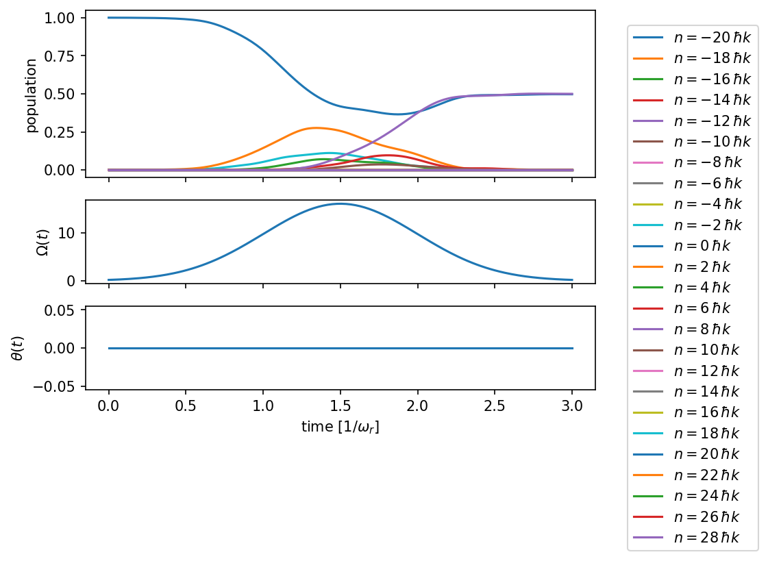
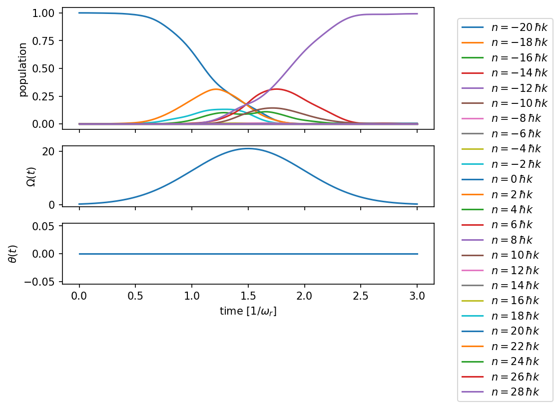
Next we can use the mwave.integrate.propagate() function to integrate some initial momentum state through a Bragg diffraction beamsplitter and mirror. We will just eyeball the effective Rabi frequencies for each.

propagate() takes the momentum grid, initial state, final time, two-photon detuning, and callable functions for the Rabi envelope and drive phase. For a Gaussian pulse we use the built-in omega_fnc_gaussian() and phase_fnc_constant().

n0, nf = 0, 4
sigma = 0.5
omega_bs = 16.1
omega_mirror = 21
kvec, n0_idx, nf_idx = mint.make_kvec(n0, nf)

# Simulate beamsplitter (pi/2 pulse)
result = mint.propagate(kvec, mint.make_phi(kvec, n0), 6*sigma, 4*(n0+nf),
                        mint.omega_fnc_gaussian, np.array([omega_bs, sigma, 3*sigma]),
                        mint.phase_fnc_constant, np.array([0.0]))
result.plot()
plt.show()

# Simulate mirror (pi pulse)
result = mint.propagate(kvec, mint.make_phi(kvec, n0), 6*sigma, 4*(n0+nf),
                        mint.omega_fnc_gaussian, np.array([omega_mirror, sigma, 3*sigma]),
                        mint.phase_fnc_constant, np.array([0.0]))
result.plot()
plt.show()

The plot() method produces a three-panel figure showing the population in each momentum state, the Rabi frequency profile, and the drive phase as a function of time.

The population at any specific momentum state can also be queried with population():

print(f"Population in n={nf}: {result.population(2*nf):.4f}")

That seems to have worked well enough!

See the Integrating the Bloch Hamiltonian section for other examples of evolving wavefunctions under the Bloch Hamiltonian.

Numeric interferometer usage

First we need to import the needed libraries and define our interferometer geometry.

import numpy as np
from matplotlib import pyplot as plt
from tqdm import tqdm

from mwave.numeric import NumericBraggInterferometer
from mwave.integrate import propagate, omega_fnc_gaussian, multi_omega_fnc, phase_fnc_constant
from mwave.utils.cloud import cloud_init
from mwave.utils.units import recoil

# Set interferometer parameters
nbragg = 4
T = recoil.time(100e-3)
Tp = recoil.time(8e-3)

# Initialize kvec and tree
ifr = NumericBraggInterferometer(-2*nbragg, 4*nbragg, distance=0) # Should pass in wavefunction initialization functions

# Define interferometer sequence
ifr.split(nbragg) # Should pass in the relevant function here as well! Function will inspect input function arguments to ensure correct number and naming
ifr.propagate(T)
ifr.split(nbragg)
ifr.propagate(Tp)
ifr.split([3*nbragg, -nbragg])
ifr.propagate(T)
ifr.split([3*nbragg, -nbragg])

# Get nodes and plot trajectories
nodes = ifr.get_nodes(x_tolerance=1e-11)
nA, nB, nC, nD = nodes[4*nbragg], nodes[2*nbragg], nodes[0.0*nbragg], nodes[-2*nbragg]
Ts = [0, 0, T, T, T + Tp, T + Tp, T + Tp + T, T + Tp + T]

plt.figure()
for nn in [nA, nB, nC, nD]:
    for p in nn:
        for node in nn[p]:
            t, x = node.get_trajectory()
            plt.plot(t, x)
plt.show()

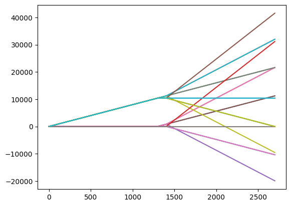
This is our SCI along with all junk ports. To calculate the phase of the interferometer numerically we need a function with signature function(*args, k_init, k_final, klattice, t, z) to pass to the ifr.compile function. This function must compute the wavefunction amplitude in state k_final resulting from a Bragg transition with lattice at klattice for initial momentum state k_init at time t and position z. For now we will ignore the position. The function we write won’t be completely general–it will only work for the values of klattice that we expect. Because of this, we will throw an error if we get an unexpected klattice value. Finally, we will define a function that acts as an “ideal” beamsplitter, and a function that actually integrates the Bragg dynamics.

# Define simulation parameters
Omega0 = 19.5
tol = 1e-6
tau_factor = 3
sigma = recoil.time(20e-6)
w0 = recoil.length(6.2e-3)

bs_lookup_dict = {}

def deltalookup(vz):
    # vz is in recoil velocity units, so it enters delta directly
    return 4*nbragg + 4*vz

def omegalookup(x, y):
    return Omega0*np.exp(-2*(x**2 + y**2)/(w0**2))

# Define beamsplitter function
def prop_bs_wavefunction_ideal(idx, x0, y0, vz, vx, vy, delta_phase_shift, omega_m, k_init, k_final, klattice, t, z):

    # Check if this is a multifrequency beamsplitter
    multifrequency = isinstance(klattice, list)

    # Check that this is a valid lattice
    if not multifrequency:
        assert klattice == nbragg
    else:
        assert len(klattice) == 2
        assert 3*nbragg in klattice
        assert -nbragg in klattice

    # Determine index of k_final state
    kf_idx = np.argmin(np.abs(ifr.kvec - k_final))

    # Determine atom number
    natoms = len(x0)

    # Return analtyic wavefunction amplitude
    if (k_final == 2*nbragg and k_init == 0) or (k_init == 2*nbragg and k_final == 0):
        return 1.0j/np.sqrt(2)*np.exp(1.0j*(-4*nbragg*t + delta_phase_shift)*(k_final - k_init)/2)
    elif (k_final == 4*nbragg and k_init == 2*nbragg) or (k_final == 2*nbragg and k_init == 4*nbragg):
        return 1.0j/np.sqrt(2)*np.exp(1.0j*(-(4*nbragg + omega_m)*t + delta_phase_shift)*(k_final - k_init)/2)
    elif (k_final == -2*nbragg and k_init == 0) or (k_final == 0 and k_init == -2*nbragg):
        return 1.0j/np.sqrt(2)*np.exp(1.0j*(-(4*nbragg - omega_m)*t + delta_phase_shift)*(k_final - k_init)/2)
    elif k_init == k_final:
        return 1.0/np.sqrt(2) + 0.0j
    else:
        return 0.0 + 0.0j

# Define beamsplitter function
def prop_bs_wavefunction_bragg(idx, x0, y0, vz, vx, vy, delta_phase_shift, omega_m, k_init, k_final, klattice, t, z):

    # Check if this is a multifrequency beamsplitter
    multifrequency = isinstance(klattice, list)

    # Check that this is a valid lattice
    if not multifrequency:
        assert klattice == nbragg
    else:
        assert len(klattice) == 2
        assert 3*nbragg in klattice
        assert -nbragg in klattice

    # Determine index of k_final state
    k0_idx = np.argmin(np.abs(ifr.kvec - k_init))
    kf_idx = np.argmin(np.abs(ifr.kvec - k_final))

    # Determine atom number
    natoms = len(x0)
    # Load cached result
    if idx in bs_lookup_dict:
        if k_init in bs_lookup_dict[idx]:
            return bs_lookup_dict[idx][k_init][:, kf_idx] if natoms > 1 else bs_lookup_dict[idx][k_init][kf_idx]

    # Compute omegas and deltas
    x = x0 + vx*t
    y = y0 + vy*t
    omegas = omegalookup(x, y)
    deltas = deltalookup(vz)

    # Create phi0
    phi0 = np.zeros_like(ifr.kvec, dtype=np.complex128)
    phi0[k0_idx] = 1.0 + 0.0j

    if natoms > 1:
        phi0 = np.tile(phi0, (natoms, 1))
    else:
        deltas = deltas[0]
        omegas = omegas[0]

    # Integrate
    if not multifrequency:
        result = propagate(
            ifr.kvec, phi0, t + 2*tau_factor*sigma, deltas,
            omega_fnc_gaussian, np.array([1.0, sigma, t + tau_factor*sigma]),
            phase_fnc_constant, np.array([delta_phase_shift]),
            omegas=omegas, t0=t, tol=tol
        )
    else:
        result = propagate(
            ifr.kvec, phi0, t + 2*tau_factor*sigma, deltas,
            multi_omega_fnc, np.array([1.0, sigma, t + tau_factor*sigma, omega_m]),
            phase_fnc_constant, np.array([delta_phase_shift]),
            omegas=omegas, t0=t, tol=tol
        )

    # Save result
    phi = result.phi_final

    # Save wavefunction to cache
    if idx not in bs_lookup_dict:
        bs_lookup_dict[idx] = {}
    if k_init not in bs_lookup_dict[idx]:
        bs_lookup_dict[idx][k_init] = phi
    else:
        raise RuntimeError('Array should not have been created but it was!')

    # Return
    return bs_lookup_dict[idx][k_init][:, kf_idx] if natoms > 1 else bs_lookup_dict[idx][k_init][kf_idx]

Now we will compile the interferometer using the function we have defined above along with the function that describes how phase accumulates during free propagation (this is a trivial function). The NumericBraggInterferometer class will automatically call the beamsplitter function we have defined at each split, and the propagation function during the propagation steps. We will wrap the compile function in a function called sim_ellipse that accepts a phase (supposedly coming from vibrations that shift the phase of the third Bragg pulse), and a modulation frequency. It will return the x and y location of the ellipse shot for the provided vibration_phase and omega_m.

def sim_ellipse(vibration_phase, omega_m, use_ideal=False):

    prop_bs_wavefunction = prop_bs_wavefunction_ideal if use_ideal else prop_bs_wavefunction_bragg

    split_funcs = [
        lambda x0, y0, vz, vx, vy, k_init, k_final, klattice, t, z: prop_bs_wavefunction(0, x0, y0, vz, vx, vy, 0.0, omega_m, k_init, k_final, klattice, t, z),
        lambda x0, y0, vz, vx, vy, k_init, k_final, klattice, t, z: prop_bs_wavefunction(1, x0, y0, vz, vx, vy, 0.0, omega_m, k_init, k_final, klattice, t, z),
        lambda x0, y0, vz, vx, vy, k_init, k_final, klattice, t, z: prop_bs_wavefunction(2, x0, y0, vz, vx, vy, vibration_phase, omega_m, k_init, k_final, klattice, t, z),
        lambda x0, y0, vz, vx, vy, k_init, k_final, klattice, t, z: prop_bs_wavefunction(3, x0, y0, vz, vx, vy, 0.0, omega_m, k_init, k_final, klattice, t, z)
    ]

    propagate_func = lambda x0, y0, vz, vx, vy, t, k: np.exp(-1j*t*k**2)

    kvector_funcs = [
        lambda x0, y0, vz, vx, vy, k_init, k_final, klattice, t, z: 0.0,
        lambda x0, y0, vz, vx, vy, k_init, k_final, klattice, t, z: 0.0,
        lambda x0, y0, vz, vx, vy, k_init, k_final, klattice, t, z: 0.0,
        lambda x0, y0, vz, vx, vy, k_init, k_final, klattice, t, z: 0.0,
    ]

    output_momenta = [4*nbragg, 2*nbragg, 0*nbragg, -2*nbragg]

    popfunc = ifr.compile(split_funcs=split_funcs,
                        propagate_func=propagate_func,
                        output_momentums=output_momenta,
                        kvector_funcs=kvector_funcs,
                        x_tolerance=1e-11)

    def xyfunc(x0, y0, vz, vx, vy):
        pA, pB, pC, pD = popfunc(4*nbragg, [x0, y0, vz, vx, vy]), popfunc(2*nbragg, [x0, y0, vz, vx, vy]), popfunc(0*nbragg, [x0, y0, vz, vx, vy]), popfunc(-2*nbragg, [x0, y0, vz, vx, vy])
        return (pB-pA)/(pB+pA), (pD-pC)/(pD+pC)

    # Cloud parameters supplied in recoil units: lengths in L_r, velocities in v_r
    x0, y0, z0, vz, vx, vy = cloud_init(natoms=1000, sigma_cloud=recoil.length(1e-3), sigma_transverse_v=1.5, sigma_vertical_v=0.1, seed=137)
    x, y = xyfunc(x0, y0, vz, vx, vy)
    x, y = np.mean(x), np.mean(y)

    return x, y

Now, keeping the vibration phase fixed, we will scan the modulation frequency for the ideal beamsplitter case. From Brian Estey’s thesis Eq.(2.27) and the unlabeled equation preceeding Eq.(2.27) we also know what phase we expect analytically for both x and y. We plot these alongside the numerically computed phase.

# Define analytic form of x and y
def analytic_ellipse(vibration_phase, omega_m):
    phid = 8*nbragg**2*T - nbragg*omega_m*T
    phic = vibration_phase
    pA = np.cos((phic+phid)/2)**2/8
    pB = np.cos((phic-phid)/2)**2/8
    pC = np.sin((phic-phid)/2)**2/8
    pD = np.sin((phic+phid)/2)**2/8
    return (pB-pA)/(pB+pA)/2, (pD-pC)/(pD+pC)/2

# Define phases to scan over
target_phases = np.linspace(-2*np.pi, 2*np.pi, 16)
omega_ms = 8*nbragg + target_phases/(2*nbragg*T)

# Loop over each modulation frequency, compute x and y
x, y = np.full_like(omega_ms, np.nan), np.full_like(omega_ms, np.nan)
ax, ay = np.full_like(omega_ms, np.nan), np.full_like(omega_ms, np.nan)
for i in tqdm(range(len(omega_ms))):
    bs_lookup_dict = {} # Reset cache
    x[i], y[i] = sim_ellipse(0.0, omega_ms[i], use_ideal=True)
    ax[i], ay[i] = analytic_ellipse(np.pi/2, omega_ms[i])

# Plot
plt.plot(target_phases/np.pi, x, label='sim x')
plt.plot(target_phases/np.pi, y, label='sim y')
plt.plot(target_phases/np.pi, ax, '--', label='analytic x')
plt.plot(target_phases/np.pi, ay, '--', label='analytic y')
plt.legend()
plt.show()

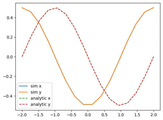
The periods agree, but it seems we have a phase offset of \(\pi/4\) between the two. Not sure why this is.

Moving along to an ellipse

# Define phases to scan over, select opening phase of pi/2
omega_m = 8*nbragg - np.pi/2/(2*nbragg*T)
vibration_phases = np.linspace(0, 2*np.pi/nbragg, 16)

# Loop over each vibration phase, compute x and y
x, y = np.full_like(vibration_phases, np.nan), np.full_like(vibration_phases, np.nan)
ax, ay = np.full_like(omega_ms, np.nan), np.full_like(omega_ms, np.nan)
for i in tqdm(range(len(vibration_phases))):
    bs_lookup_dict = {}
    x[i], y[i] = sim_ellipse(vibration_phases[i], omega_m, use_ideal=True)
    ax[i], ay[i] = analytic_ellipse(np.pi/2, omega_ms[i])

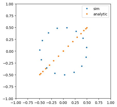
plt.plot(x, y, '.', label='sim')
plt.plot(ax, ay, '.', label='analytic')
plt.xlim(-1,1)
plt.ylim(-1,1)
plt.legend()
plt.gca().set_aspect('equal')
plt.show()