Interferometer Geometries

Mach-Zender Interferometer

Define the needed constants, initialize the required unitary operators, and define the interferometer.

from mwave import symbolic as msym
import numpy as np
import sympy as sp
from matplotlib import pyplot as plt

# Set up symbols for symbolic computation
m, c, hbar, k, g, gamma, delta, n, T, t_traj = sp.symbols('m c hbar k g gamma delta n T t_traj', real=True)
k_eff = 2*k

# Register constants
msym.set_constants(m=m, c=c, hbar=hbar, t_traj=t_traj)

# Define unitary operators needed for an MZ interferometer
bs = msym.Beamsplitter(0, n, delta, k_eff)
mirror = msym.Mirror(0, n, delta, k_eff)
free = msym.FreeEv(T, gravity=g, gravity_grad=gamma)

# Create interferometer object, perform MZ sequence
ifr = msym.Interferometer()
(bs @ (free @ (mirror @ (free @ (bs @ ifr)))))

<mwave.symbolic.Interferometer at 0x18bffa307d0>

Generate and optionally vizualize the directed tree structure representing the interferometer object.

# Create a graphviz object of the tree
d_test = ifr.generate_graph()

# Uncomment to display the graph
# d_test.view()

Check for interferance, set the gravity gradient to zero as otherwise the interferometer won’t perfectly close and no interferance will be detected.

inodes = ifr.interfere(subs={gamma: 0})

Determine which port each output is in

iports, jports, noport = ifr.get_ports({n:'upper', 0: 'lower'})

Check that we don’t have any unexpected ports

if len(jports) != 0 or len(noport) != 0:
    print('Unexpected output')

Set interferometer parameters for plotting

subs = {m: 1, c: 1, hbar: 1, k: 1, g: 0.3, gamma: 0.001, delta: 4*3, n: 3, T: 5}

Determine the final interferometer time by evaluating the value of t at the end of the interferometer. We can pick a random interferometer port to do this.

tfinal = float(iports['upper'][0].t.evalf(subs=subs))

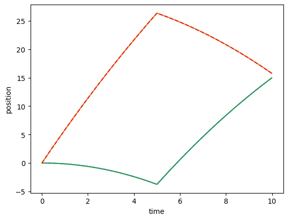
Plot the trajectory of the interferometer paths

t = np.linspace(0, tfinal, 1000)
plt.figure()
for node_pair, ls in zip([iports['upper'], iports['lower']], ['-', '--']):
    fnc_traj = node_pair[0].get_trajectory(subs=subs)
    plt.plot(t, fnc_traj(t), linestyle=ls)
    fnc_traj = node_pair[1].get_trajectory(subs=subs)
    plt.plot(t, fnc_traj(t), linestyle=ls)
plt.xlabel('time')
plt.ylabel('position')
plt.show()

Compute the phase of the interferometer

# Compute the differential phase
phi1, phi2 = ifr.phases()
print(f'phase_1={sp.simplify(phi1)}')
print(f'phase_2={sp.simplify(phi2)}')

# Print out the total population, check it is equal to 1
pop = 0
for node in ifr.get_nodes():
    pop += (node.get_amp())**2
print(f'total population sum={sp.simplify(pop)}')

phase_1=(-3*T**10*g*gamma**4*k*m*n + 10*T**9*gamma**4*hbar*k**2*n**2 - 34*T**8*g*gamma**3*k*m*n + 56*T**7*gamma**3*hbar*k**2*n**2 - 53*T**6*g*gamma**2*k*m*n + 60*T**5*gamma**2*hbar*k**2*n**2 + 84*T**4*g*gamma*k*m*n - 144*T**3*gamma*hbar*k**2*n**2 + 144*T**2*g*k*m*n - 72*pi*m)/(72*m)
phase_2=T**2*k*n*(-3*T**8*g*gamma**4*m + 10*T**7*gamma**4*hbar*k*n - 34*T**6*g*gamma**3*m + 56*T**5*gamma**3*hbar*k*n - 53*T**4*g*gamma**2*m + 60*T**3*gamma**2*hbar*k*n + 84*T**2*g*gamma*m - 144*T*gamma*hbar*k*n + 144*g*m)/(72*m)
total population sum=1

Simultaneous Conjugate Interferometer

Define the needed constants, initialize the required unitary operators, and define the interferometer.

from mwave import symbolic as msym
import numpy as np
import sympy as sp
from matplotlib import pyplot as plt

# Set up symbols for symbolic computation
m, c, hbar, k, omega_r, delta, n, omega_m, T, Tp, t_traj = sp.symbols('m c hbar k omega_r delta n omega_m T Tp t_traj', real=True)
k_eff = 2*k

# Register constants
msym.set_constants(m=m, c=c, hbar=hbar, t_traj=t_traj)

# Define unitary operators needed for an SCI interferometer
bs1 = msym.Beamsplitter(n, 0, delta, k_eff)
bs2 = msym.Beamsplitter(0, -n, delta - omega_m, k_eff)
bs2u = msym.Beamsplitter(n, 2*n, delta + omega_m, k_eff)
fe1 = msym.FreeEv(T)
fe2 = msym.FreeEv(Tp)

# Create interferometer object, perform MZ sequence
ifr = msym.Interferometer()
ifr.apply(bs1)
ifr.apply(fe1)
ifr.apply(bs1)
ifr.apply(fe2)
ifr.apply(bs2)
ifr.apply(bs2u)
ifr.apply(fe1)
ifr.apply(bs2)
ifr.apply(bs2u)

Generate and optionally vizualize the directed tree structure representing the interferometer object.

# Create a graphviz object of the tree
d_test = ifr.generate_graph()

# Uncomment to display the graph
# d_test.view()

Check for interferance, set the gravity gradient to zero as otherwise the interferometer won’t perfectly close and no interferance will be detected.

inodes = ifr.interfere()

Determine which port each output is in

iports, jports, noport = ifr.get_ports({2*n:'A', n:'B', 0:'C', -n:'D'})

Check that we don’t have any unexpected ports

if len(jports) != 4 or len(noport) != 0:
    print('Unexpected output')

Set interferometer parameters for plotting

subs = {m: 1, c: 1, hbar: 1, k: 1, delta: 4*3, n: 3, T: 5, Tp: 1}

Determine the final interferometer time by evaluating the value of t at the end of the interferometer. We can pick a random interferometer port to do this.

tfinal = float(iports['A'][0].t.evalf(subs=subs))

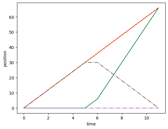
Plot the trajectory of the interferometer paths

t = np.linspace(0, tfinal, 1000)
plt.figure()
for port, ls in zip(['A', 'B', 'C', 'D'], ['-', '--', '-.', ':']):
    fnc_traj = iports[port][0].get_trajectory(subs=subs)
    plt.plot(t, fnc_traj(t), linestyle=ls)
    fnc_traj = iports[port][1].get_trajectory(subs=subs)
    plt.plot(t, fnc_traj(t), linestyle=ls)
plt.xlabel('time')
plt.ylabel('position')
plt.show()

Compute the phase of the interferometer

# Compute the differential phase
phiA, phiB, phiC, phiD = ifr.phases()
print(f'differential phase={sp.simplify(phiA - phiC).subs(k, sp.sqrt(2*m*omega_r/hbar))}')

# Print out the total population, check it is equal to 1
pop = 0
for node in ifr.get_nodes():
    pop += (node.get_amp())**2
print(f'total population sum={sp.simplify(pop)}')

differential phase=16*T*n**2*omega_r - 2*T*n*omega_m - 2*pi
total population sum=1

Simulatenous Conjugate Interferometer with single Bragg pulses

from mwave import symbolic as msym
import numpy as np
import sympy as sp
from matplotlib import pyplot as plt

# Set up symbols for symbolic computation
k, c, hbar, m, g, T_spacing, T, Tp, delta, t_traj, omega_r, omega_0 = sp.symbols('k c hbar m g T_spacing T Tp delta t_traj omega_r omega_0', real=True)
k_eff = 2*k

# Register constants
msym.set_constants(m=m, c=c, hbar=hbar, t_traj=t_traj)

For an n=2 SCI with single Bragg pulses we must run the following pulse sequences for beam splitters

Pulse sequence 1: Split initial state into two, mirror one of the outputs to bragg order n
1       2     ...    n
pi/2 -> pi -> ... -> pi

Pulse sequence 2: Mirror state at momentum n down to 1, then pi/2 to bring to correct state and diffract initially undiffracted arm to 1, then mirror initially undiffracted arm up to n
1            n-1   n       n+1          n+n-1
pi -> ... -> pi -> pi/2 -> pi -> ... -> pi

Pulse sequence 3: pi/2 lower interferometer upper arm down (pi/2 necessary to avoid diffracting away the lower arm), pi pulse to -n. Simulaneously do the same for the upper interferometer lower arm
1       2            n
pi/2 -> pi -> ... -> pi

Pulse sequence 4: pi lower interferometer upper arm up to 0, pi/2 pulse to interfere 0 and -1 states. Simulaneously do the same for the upper interferometer lower arm
1            2     n
pi -> ... -> pi -> pi/2

We will next implement the unitary operators needed to perform these sequences

nbragg = 2

bsdict = {}
mdict = {}

# Make function to get/construct a beamsplitter between the two specified states
def get_bs(n0, nf):
    tid = (min(n0,nf), max(n0,nf))
    if tid in bsdict:
        return bsdict[tid]
    else:
        bsdict[tid] = msym.Beamsplitter(min(n0,nf), max(n0,nf), 4*(n0+nf)*omega_0, k_eff)
        return bsdict[tid]

# Make function to get/construct a mirror between the two specified states
def get_m(n0, nf):
    tid = (min(n0,nf), max(n0,nf))
    if tid in mdict:
        return mdict[tid]
    else:
        mdict[tid] = msym.Mirror(min(n0,nf), max(n0,nf), 4*(n0+nf)*omega_0, k_eff)
        return mdict[tid]

# Free evolutions
feTs = msym.FreeEv(T_spacing)
feT = msym.FreeEv(T)
feTp = msym.FreeEv(Tp)

# Beamsplitter sequences
def pulse1(ifr):
    ifr.apply(get_bs(0, 1))
    for n in range(1, nbragg):
        ifr.apply(feTs)
        ifr.apply(get_m(n, n+1))

def pulse2(ifr):
    for n in range(nbragg, 1, -1):
        ifr.apply(get_m(n, n-1))
        ifr.apply(feTs)
    ifr.apply(get_bs(1, 0))
    for n in range(1, nbragg):
        ifr.apply(feTs)
        ifr.apply(get_m(n, n+1))

def pulse3(ifr):
    ifr.apply(get_bs(0, -1))
    ifr.apply(get_bs(nbragg, nbragg+1))
    for n in range(1, nbragg):
        ifr.apply(feTs)
        ifr.apply(get_m(-n, -n-1))
        ifr.apply(get_m(nbragg+n, nbragg+n+1))

def pulse4(ifr):
    for n in range(nbragg, 1, -1):
        ifr.apply(get_m(-n, -n+1))
        ifr.apply(get_m(nbragg+n, nbragg+n-1))
        ifr.apply(feTs)
    ifr.apply(get_bs(0, -1))
    ifr.apply(get_bs(nbragg, nbragg+1))

Create the interferometer object and apply our sequence of unitary operators

ifr = msym.Interferometer()
pulse1(ifr)
ifr.apply(feT)
pulse2(ifr)
ifr.apply(feTp)
pulse3(ifr)
ifr.apply(feT)
pulse4(ifr)

Generate and optionally vizualize the directed tree structure representing the interferometer object.

# Create a graphviz object of the tree
d_test = ifr.generate_graph()

# Uncomment to display the graph
# d_test.view()

Check for interferance, set the gravity gradient to zero as otherwise the interferometer won’t perfectly close and no interferance will be detected.

inodes = ifr.interfere()

Determine which port each output is in

iports, jports, noport = ifr.get_ports({nbragg+1:'A', nbragg:'B', 0:'C', -1:'D'})

Check that we don’t have any unexpected ports

if len(jports) != 4 or len(noport) != 0:
    print('Unexpected output')

Set interferometer parameters for plotting

subs = {k: 2, c: 1, hbar: 1, m: 1, T_spacing: 1, delta: 4*omega_r, omega_r: 1, T:5, Tp: 3, g: 1}

Determine the final interferometer time by evaluating the value of t at the end of the interferometer. We can pick a random interferometer port to do this.

tfinal = float(inodes[0][0].t.evalf(subs=subs))

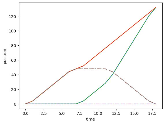
Plot the trajectory of the interferometer paths

t = np.linspace(0, tfinal, 1000)
plt.figure()
for port, ls in zip(['A', 'B', 'C', 'D'], ['-', '--', '-.', ':']):
    fnc_traj = iports[port][0].get_trajectory(subs=subs)
    plt.plot(t, fnc_traj(t), linestyle=ls)
    fnc_traj = iports[port][1].get_trajectory(subs=subs)
    plt.plot(t, fnc_traj(t), linestyle=ls)
plt.xlabel('time')
plt.ylabel('position')
plt.show()

Compute the phase of the interferometer

# Compute the differential phase
phiA, phiB, phiC, phiD = ifr.phases()
print(f'differential phase={sp.simplify(phiA - phiC).subs(k, sp.sqrt(2*m*omega_r/hbar))}')

# Print out the total population, check it is equal to 1
pop = 0
for node in ifr.get_nodes():
    pop += (node.get_amp())**2
print(f'total population sum={sp.simplify(pop)}')

differential phase=-64*T*omega_0 + 64*T*omega_r - 48*T_spacing*omega_0 + 48*T_spacing*omega_r - 2*pi
total population sum=1