Integrating the Bloch Hamiltonian

Adiabatic Bragg pulse

First lets simulate the adiabatic Bragg pulse from Adiabatic-rapid-passage multiphoton Bragg atom optics by Kovachy.

from mwave.integrate import bloch, make_kvec, make_phi
from numba import jit
import numpy as np
from matplotlib import pyplot as plt

# Define pulse parameters
n0, nf = 0, 5
omega = 30
delta = 4*(n0 + nf)

# Compute tfinal and t0 from sigma
tfinal = 8*2*np.pi
t0 = tfinal/2

# Compute detuning ramp rate as 2*omega_r/(tfinal/2)
rate = 2/(tfinal/2)

# Define pulse profile used in Kovachy (2012)
@jit(nopython=True)
def omega_fnc(t, args):
    omega = args[0]
    return omega*np.tanh(8*t/tfinal)*np.tanh(8*(1 - t/tfinal))

# Define the phase used in Kovachy (2012)
@jit(nopython=True)
def phase_fnc(t, args):
    tcurrent = (t-tfinal/2)
    return rate/2*(tcurrent**2) # The phase is the integral of the time dependent frequency over time

# Write out a function for the detuning vs time
def delta_fnc(t):
    tcurrent = (t-tfinal/2)
    return rate*tcurrent

# Define the initial state and the kvec array
kvec, n0_idx, nf_idx = make_kvec(n0, nf)
phi0 = make_phi(kvec, n0)

# Integrate the pulse
sol = bloch(kvec, phi0, tfinal, delta, omega_fnc, np.array([omega]), phase_fnc, np.array([]))

# Determine the minimum and maximum indicies
n_max = max(n0_idx, nf_idx)
n_min = min(n0_idx, nf_idx)

# Plot
fig, [ax1, ax2, ax3] = plt.subplots(nrows = 3, sharex=True, gridspec_kw={'height_ratios': [2, 1, 1]})
ax1.plot(sol.t, np.abs(sol.y.T[:,n_min-2:n_max+2])**2, label=[r"$%i\hbar k$" % k for k in kvec[n_min-2:n_max+2]])
ax2.plot(sol.t, [omega_fnc(t, np.array([omega])) for t in sol.t])
ax3.plot(sol.t, [delta_fnc(t) for t in sol.t])
ax1.legend(bbox_to_anchor=(1.05, 0.95))
ax1.set_ylabel(r'population')
ax2.set_ylabel(r'$\Omega(t)$')
ax3.set_ylabel(r'$\delta(t)$')
ax3.set_xlabel(r'time [$\omega_r$]')
fig.suptitle(r'$n_\text{bragg}=5$, $\Omega(t)=\Omega\tanh(8t/t_f)\tanh(8(1-t/t_f))$, $t_f=2\pi %0.1f$' % (tfinal/2/np.pi))
plt.show()

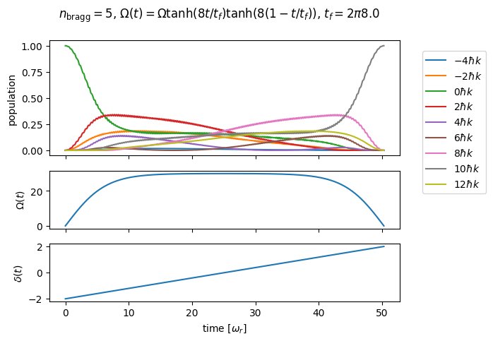
The two lower subplots are equivalent to Fig. 1a and b from the paper.

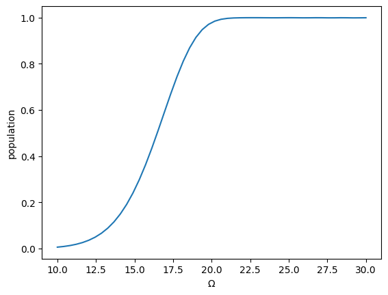
Next lets replicate Fig. 2a

# Define a function to compute the population in the final state as a function of the drive
fpop = lambda omega: np.abs(bloch(kvec, phi0, tfinal, delta, omega_fnc, np.array([omega]), phase_fnc, np.array([]), atol=1e-6, rtol=1e-6).y[nf_idx,-1])**2

# Compute along an array of omega values
omegas = np.linspace(10,30)
pops = np.full_like(omegas, np.nan)
for i in range(len(omegas)):
    pops[i] = fpop(omegas[i])

# Plot
fig, ax1 = plt.subplots()
ax1.plot(omegas, pops)
ax1.set_ylabel(r'population')
ax1.set_xlabel(r'$\Omega$')
plt.show()

Bloch oscillations

The lattice velocity should initially be that of the atoms and should be swept at rate \(\alpha\) until the lattice velocity reaches our target velocity. Mathematically this works out to be

\[\delta_0=8n_0\omega_r\]

\[\delta(t)=\delta_0+\alpha t\]

\[\delta_f=8n_f\omega_r\]

The phase of the drive is therefore

\[\theta(t)=\delta_0t+\frac{1}{2}\alpha t^2\]

The sweep should be stopped at

\[t_f=(\delta_f-\delta_0)/\alpha=8(n_f-n_0)\omega_r/\alpha\]

Lets try this out with fifth order Bloch

from mwave.integrate import bloch, make_kvec, make_phi
from numba import jit
import numpy as np
from matplotlib import pyplot as plt

# Define pulse parameters
n0, nf = 0, 5
omega = 2
alpha = 1

# Compute parameters
delta0 = 8*n0
deltaf = 8*nf
tfinal = (deltaf-delta0)/alpha

# Define a constant pulse profile
@jit(nopython=True)
def omega_fnc(t, args):
    omega = args[0]
    return omega

# Define a quadratically ramped phase
@jit(nopython=True)
def phase_fnc(t, args):
    return delta0*t+0.5*alpha*t**2 # The phase is the integral of the time dependent frequency over time

# Write out a function for the detuning vs time
def delta_fnc(t):
    return delta0+alpha*t

# Define the initial state and the kvec array
kvec, n0_idx, nf_idx = make_kvec(n0, nf)
phi0 = make_phi(kvec, n0)

# Integrate the pulse
sol = bloch(kvec, phi0, tfinal, 0, omega_fnc, np.array([omega]), phase_fnc, np.array([]))

# Determine the minimum and maximum indicies
n_max = max(n0_idx, nf_idx)
n_min = min(n0_idx, nf_idx)

# Plot
fig, [ax1, ax2, ax3] = plt.subplots(nrows = 3, sharex=True, gridspec_kw={'height_ratios': [2, 1, 1]})
ax1.plot(sol.t, np.abs(sol.y.T[:,n_min-2:n_max+2])**2, label=[r"$%i\hbar k$" % k for k in kvec[n_min-2:n_max+2]])
ax2.plot(sol.t, [omega_fnc(t, np.array([omega])) for t in sol.t])
ax3.plot(sol.t, [delta_fnc(t) for t in sol.t])
ax1.legend(bbox_to_anchor=(1.05, 0.95))
ax1.set_ylabel(r'population')
ax2.set_ylabel(r'$\Omega(t)$')
ax3.set_ylabel(r'$\delta(t)$')
ax3.set_xlabel(r'time [$\omega_r$]')
plt.show()

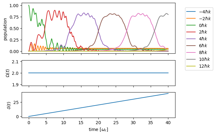
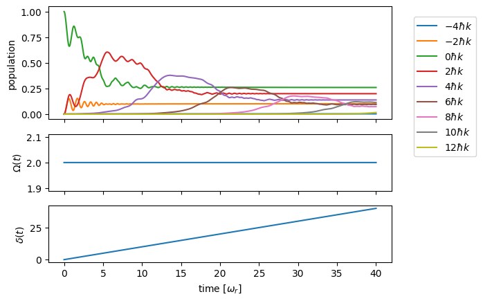
There we go! Note that this simulation does not include any effect of loading the lattice, etc.

We can easily account for single photon scattering by including the Gamma_sps parameter in our call to the mwave.integrate.bloch() function. This causes mwave.integrate.bloch() to integrate the density matrix instead of the wavefunction.

from mwave.integrate import bloch, make_kvec, make_phi
from numba import jit
import numpy as np
from matplotlib import pyplot as plt

# Define pulse parameters
n0, nf = 0, 5
omega = 2
alpha = 1
Gamma_sps = 0.5

# Compute parameters
delta0 = 8*n0
deltaf = 8*nf
tfinal = (deltaf-delta0)/alpha

# Define a constant pulse profile
@jit(nopython=True)
def omega_fnc(t, args):
    omega = args[0]
    return omega

# Define a quadratically ramped phase
@jit(nopython=True)
def phase_fnc(t, args):
    return delta0*t+0.5*alpha*t**2 # The phase is the integral of the time dependent frequency over time

# Write out a function for the detuning vs time
def delta_fnc(t):
    return delta0+alpha*t

# Define the initial state and the kvec array
kvec, n0_idx, nf_idx = make_kvec(n0, nf)
phi0 = make_phi(kvec, n0)

# Integrate the pulse
sol = bloch(kvec, phi0, tfinal, 0, omega_fnc, np.array([omega]), phase_fnc, np.array([]), Gamma_sps=Gamma_sps)
pops = np.diagonal(sol.y)

# Determine the minimum and maximum indicies
n_max = max(n0_idx, nf_idx)
n_min = min(n0_idx, nf_idx)

# Plot
fig, [ax1, ax2, ax3] = plt.subplots(nrows = 3, sharex=True, gridspec_kw={'height_ratios': [2, 1, 1]})
ax1.plot(sol.t, np.real(pops[:,n_min-2:n_max+2]), label=[r"$%i\hbar k$" % k for k in kvec[n_min-2:n_max+2]])
ax2.plot(sol.t, [omega_fnc(t, np.array([omega])) for t in sol.t])
ax3.plot(sol.t, [delta_fnc(t) for t in sol.t])
ax1.legend(bbox_to_anchor=(1.05, 0.95))
ax1.set_ylabel(r'population')
ax2.set_ylabel(r'$\Omega(t)$')
ax3.set_ylabel(r'$\delta(t)$')
ax3.set_xlabel(r'time [$\omega_r$]')
plt.show()