Quickstart
mwave is a python library designed to help explore new matterwave interferometer geometries. mwave also provides functions to numerically solve the Hamiltonian that describes Bragg diffraction and Bloch oscillations.
Installation
Stable releases of mwave can be downloaded from Github or via:
pip install git+https://github.com/jc-roth/mwave@v3.0.0
A first example
Defining an interferometer geometry
mwave is losely broken up into three parts: a module for symbolically defining arbitrary interferometer geometries, a module for numerically defining arbitrary interferometer geometries, and a module for numerically integrating Bragg and Bloch processes. As an example we will use the library to explore a Mach-Zender interferometer geometry.
First we will import the required libraries
from mwave import symbolic as msym
from mwave import integrate as mint
import numpy as np
import sympy as sp
from matplotlib import pyplot as plt
mwave internally uses the sympy library to build symbolic expressions of
the interferometer phase. Therefore we must define the symbols we want
to use symbolically
m, c, hbar, k, g, delta, n, T, t_traj = sp.symbols('m c hbar k g delta n T t_traj', real=True)
k_eff = 2*k
Performing certain operations in mwave requires the user to set certain
constants. In this example we will need to set the mass, speed of light,
the Planck constant, and another variable called t_traj.
msym.set_constants(m=m, c=c, hbar=hbar, t_traj=t_traj)
The unitary operators that we will use to build the interferometer
require these constants. If they are not provided an error will be
thrown. At first glance it makes sense that we need to define constants representing the mass, speed of
light, and the Planck constant in order to define our unitary operators. mwave also provides the ability to compute the position of each interferometer path as a function of time, and t_traj is used to parameterize this time.
Now we are ready to define unitary operators representing the beamsplitter, free evolution, and mirror that make up the Mach-Zender interferometer:
beamsplitter = msym.Beamsplitter(0, n, delta, k_eff, include_half_pi_shift=True)
mirror = msym.Mirror(0, n, delta, k_eff)
free = msym.FreeEv(T, gravity=g)
Now that we have defined our unitary operators we can define a new interferometer object and apply our unitary operators to it.
ifr = msym.Interferometer()
ifr.apply(beamsplitter)
ifr.apply(free)
ifr.apply(beamsplitter)
ifr.apply(free)
ifr.apply(beamsplitter)
Thats it! We have defined the full Mach-Zender interferometer! Note that
unitary operators can also be applied using the matrix multiplication
operator, i.e. free @ (beamsplitter @ ifr).
Now lets compute the phase of the interferometer. To do this we must
first call the mwave.symbolic.Interferometer.interfere() method to
check which interferometer paths interfere.
interfering_paths = ifr.interfere()
print(f'Found {len(interfering_paths)} interfering paths.')
Found 2 interfering paths.
This is expected as a Mach-Zender interferometer has two output ports.
Now that we have computed the interfering paths we can compute the phase difference between each interfering output:
phase_differences = ifr.phases()
for phase_difference in phase_differences:
    print(sp.simplify(phase_difference))
2*T**2*g*k*n - pi
2*T**2*g*k*n
See the Interferometer Geometries section for more in-depth examples of how to define and analyze interferometer geometries.
Simulating Bragg beamsplitters
Next we can use the mwave.integrate.propagate() function to integrate some initial momentum state through a Bragg diffraction beamsplitter and mirror. We will just eyeball the effective Rabi frequencies for each.
propagate() takes the momentum grid, initial state, final time, two-photon detuning, and callable functions for the Rabi envelope and drive phase. For a Gaussian pulse we use the built-in omega_fnc_gaussian() and phase_fnc_constant().
n0, nf = 0, 4
sigma = 0.5
omega_bs = 16.1
omega_mirror = 21
kvec, n0_idx, nf_idx = mint.make_kvec(n0, nf)

# Simulate beamsplitter (pi/2 pulse)
result = mint.propagate(kvec, mint.make_phi(kvec, n0), 6*sigma, 4*(n0+nf),
                        mint.omega_fnc_gaussian, np.array([omega_bs, sigma, 3*sigma]),
                        mint.phase_fnc_constant, np.array([0.0]))
result.plot()
plt.show()

# Simulate mirror (pi pulse)
result = mint.propagate(kvec, mint.make_phi(kvec, n0), 6*sigma, 4*(n0+nf),
                        mint.omega_fnc_gaussian, np.array([omega_mirror, sigma, 3*sigma]),
                        mint.phase_fnc_constant, np.array([0.0]))
result.plot()
plt.show()
The plot() method produces a three-panel figure showing the population in each momentum state, the Rabi frequency profile, and the drive phase as a function of time.
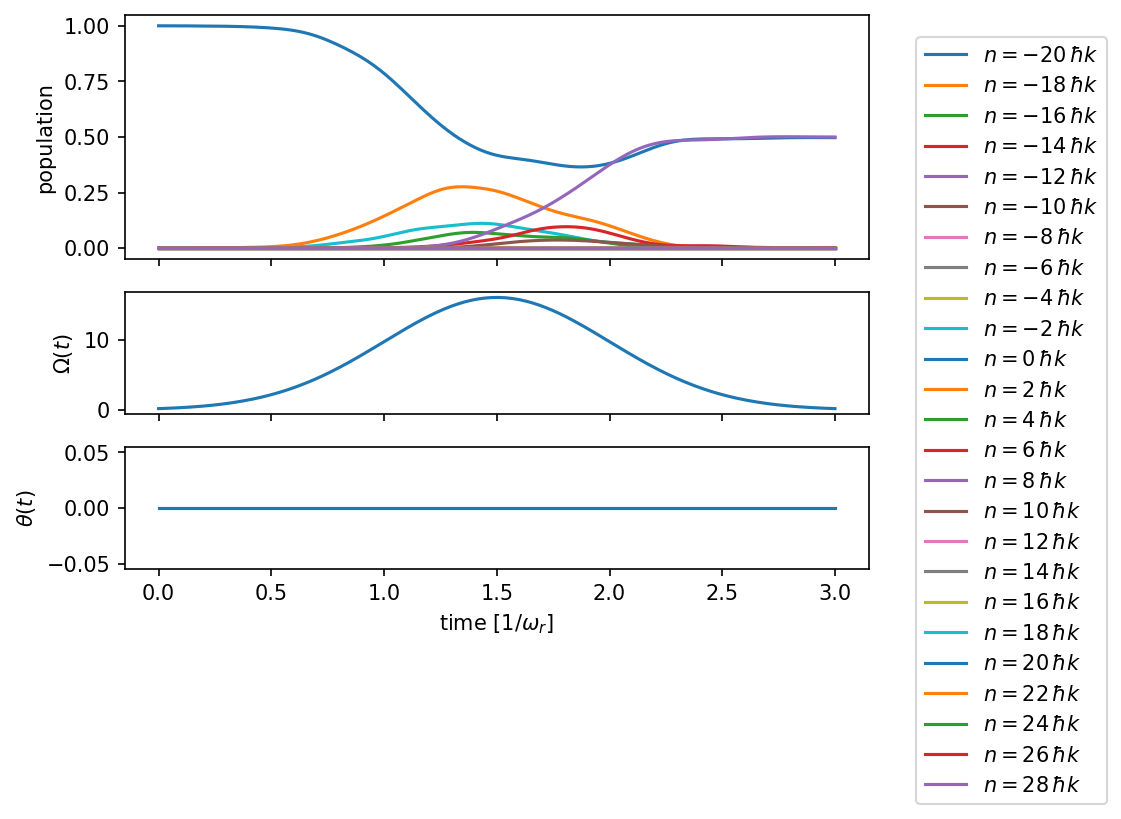
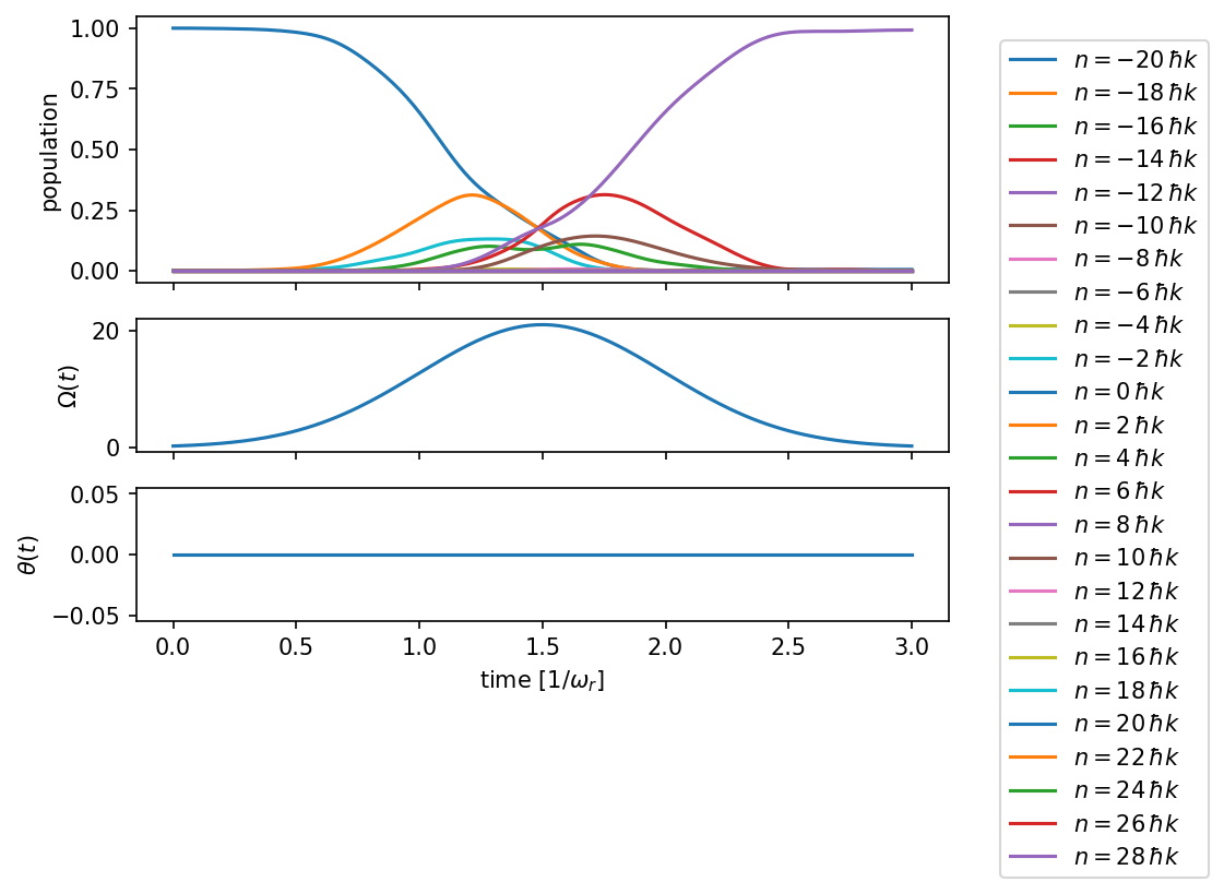
The population at any specific momentum state can also be queried with population():
print(f"Population in n={nf}: {result.population(2*nf):.4f}")
That seems to have worked well enough!
See the Integrating the Bloch Hamiltonian section for other examples of evolving wavefunctions under the Bloch Hamiltonian.
Combining the interferometer model with simulation
Note
This section describes how to integrate numeric calculations with the symbolic interferometer module. This is slightly awkward. To simulate interferometers numerically with a more natural interface please see the numeric interferometer example.
Lets say that we want to study the systematics introduced by the Bragg diffraction process in our Mach-Zender geometry. To do this we need to combine the numerical computation we’ve made using mwave.integrate.propagate() with our symbolic representation of the interferometer geometry. This is accomplished in a straightforward way by defining custom mwave.symbolic.Unitary classes that inherit from the mwave.symbolic.Beamsplitter and mwave.symbolic.Mirror classes.
Our beamsplitters will couple momentum states \(0\) and \(n\)
class BraggBeamsplitter(msym.Beamsplitter):

    def gen_numeric(self, node, subs={}):
        delta = msym.eval_sympy_var(self.delta, subs)
        kvec, _, _ = mint.make_kvec(msym.eval_sympy_var(self.n1, subs), msym.eval_sympy_var(self.n2, subs))
        n_idx = np.argmin(np.abs(2*msym.eval_sympy_var(node.n, subs) - kvec))
        n_parent = msym.eval_sympy_var(node.parent.n, subs)
        def fnc(v):
            result = mint.propagate(kvec, mint.make_phi(kvec, n_parent), 6*sigma, delta + 4*v,
                                    mint.omega_fnc_gaussian, np.array([omega_bs, sigma, 3*sigma]),
                                    mint.phase_fnc_constant, np.array([0.0]))
            return result.phi_final[n_idx]
        return fnc

class BraggMirror(msym.Mirror):

    def gen_numeric(self, node, subs={}):
        delta = msym.eval_sympy_var(self.delta, subs)
        kvec, _, _ = mint.make_kvec(msym.eval_sympy_var(self._n1, subs), msym.eval_sympy_var(self._n2, subs))
        n_idx = np.argmin(np.abs(2*msym.eval_sympy_var(node.n, subs) - kvec))
        n_parent = msym.eval_sympy_var(node.parent.n, subs)
        def fnc(v):
            result = mint.propagate(kvec, mint.make_phi(kvec, n_parent), 6*sigma, delta + 4*v,
                                    mint.omega_fnc_gaussian, np.array([omega_mirror, sigma, 3*sigma]),
                                    mint.phase_fnc_constant, np.array([0.0]))
            return result.phi_final[n_idx]
        return fnc
Now we can define new unitary operators using these definitions and apply them to an interferometer.
bragg_beamsplitter = BraggBeamsplitter(0, n, delta, k_eff)
bragg_mirror = BraggMirror(0, n, delta, k_eff)

ifr_num = msym.Interferometer()
ifr_num.apply(bragg_beamsplitter)
ifr_num.apply(free)
ifr_num.apply(bragg_mirror)
ifr_num.apply(free)
ifr_num.apply(bragg_beamsplitter)
Now we will make use of the mwave.symbolic.Interferometer.get_ports()
function to automatically map the interferometer outputs into their
respective ports.
ifr_num.interfere()
port_dict, junk_port, no_port = ifr_num.get_ports({n: 'upper', 0: 'lower'})
Now we can take the mwave.symbolic.InterferometerNode objects in
each port and generate functions that numerically calculate their
respective complex amplitudes. To generate these functions we must also
set our symbolic variables to numeric values.
subs = {hbar:1, k:1, m: 1, g: 1, n: 4, delta: 4*n, T:5}

u1 = port_dict['upper'][0].gen_numeric_wf_func(subs)
u2 = port_dict['upper'][1].gen_numeric_wf_func(subs)

l1 = port_dict['lower'][0].gen_numeric_wf_func(subs)
l2 = port_dict['lower'][1].gen_numeric_wf_func(subs)

# Create a function to compute the phase between the output wavefunctions
def calc_phase(v):
    uphase, lphase = np.angle(u1(v)/u2(v)), np.angle(l1(v)/l2(v))

    return uphase, lphase
Note that these numerically calculated complex amplitudes do not include any of the analytically derived phases.
Finally we can compute and plot how the populations vary as a function of the input particle velocity
vs = np.linspace(-0.5, 0.5, 50)
upper = np.full_like(vs, np.nan)
lower = np.full_like(vs, np.nan)

for i in range(len(vs)):
    upper[i], lower[i] = calc_phase(vs[i])

fig, [ax1, ax2] = plt.subplots(nrows=2, sharex=True)
ax1.plot(vs, upper)
ax2.plot(vs, lower)
ax2.set_xlabel('initial velocity')
ax1.set_ylabel('upper interferometer phase [rad]')
ax2.set_ylabel('lower interferometer phase [rad]')
plt.show()
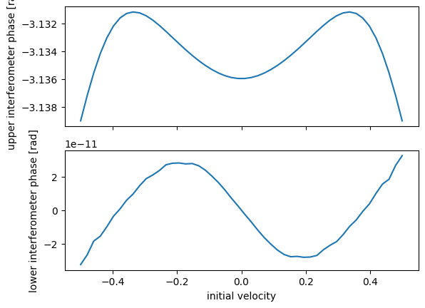
The paths that interfere in the upper output port of the interferometer do not experience the same set of beamsplitter/mirror pulses, and so they experience a phase dependent on the input velocity. The paths that interfere in the lower output port of the interferometer experience the same set of beamsplitters, and mirrors that are equivalent via a frame transformation. Therefore the imperfect phase imprinted by the Bragg process cancels out in this output port.
See the Simultaneous Conjugate Interferometer with realistic beamsplitters section for a more detailed example of how to implement the mwave.symbolic.Unitary.gen_numeric() function.
Sometimes we might be interested in having more direct control over the phases
that contribute to this numerical calculation. To help with this mwave provides the code generation function mwave.symbolic.Interferometer.generate_code_outline():
port_dict, junk_port, no_port = ifr.get_ports({n: 'upper', 0: 'lower'})
print(ifr.generate_code_outline(port_dict))
def args_lookup(x, y, v):
    return (np.ones_like(x), )

def bs(ni, nf, *args):
    if ni == nf:
        return (0.5+0j)*args[0]
    else:
        return (0+0.5j)*args[0]

def calc_populations(x0, y0, v0, ncopies):

    # Compute the ones array
    ones = np.ones(ncopies)

    # Compute positions at each beamsplitter
    x1, y1 = x0 + vx*T, y0 + vy*T
    x2, y2 = x1 + vx*T, y1 + vy*T

    # Compute velocity at each beamsplitter
    v1 = v0
    v2 = v1

    # Compute arguments at each beamsplitter
    args0 = args_lookup(x0, y0, v0)
    args1 = args_lookup(x1, y1, v1)
    args2 = args_lookup(x2, y2, v2)

    # Compute wavefunctions
    portlower_1 = bs(0,0,*args0)*bs(0,n,*args1)*bs(n,0,*args2)
    portlower_2 = bs(0,n,*args0)*bs(n,0,*args1)*bs(0,0,*args2)

    portupper_1 = bs(0,0,*args0)*bs(0,n,*args1)*bs(n,n,*args2)
    portupper_2 = bs(0,n,*args0)*bs(n,0,*args1)*bs(0,n,*args2)

    # Interfere
    portlower = np.einsum('i,j->ij', portlower_1, ones) + np.einsum('i,j->ij', portlower_2, ones)
    portupper = np.einsum('i,j->ij', portupper_1, ones) + np.einsum('i,j->ij', portupper_2, ones)

    # Compute populations
    poplower = np.sum(np.abs(portlower)**2, axis=0)
    popupper = np.sum(np.abs(portupper)**2, axis=0)

    # Return
    return poplower, popupper
We can see that this outline computes the wavefunctions output by the interferometer. We can use this outline to start incorporating additional interferometer effects.